1
2
3
4
5
6
7
8
9
10
11
12
13
14
15
16
17
18
19
20
21
22
23
24
25
26
27
28
29
30
31
32
33
34
35
36
37
38
39
40
41
42
43
44
45
46
47
48
49
50
51
52
53
54
55
56
57
58
59
60
61
62
63
64
65
66
67
68
69
70
71
72
73
74
75
76
77
78
79
80
81
82
83
84
85
86
87
88
89
90
91
92
93
94
95
96
97
98
99
100
101
102
103
104
105
106
107
108
109
110
111
112
113
114
115
116
117
118
119
120
121
122
123
124
125
126
127
128
129
130
131
132
133
134
135
136
137
138
139
140
141
142
143
144
145
146
147
148
149
150
151
152
153
154
155
156
157
158
159
160
161
162
163
164
165
166
167
168
169
170
171
172
173
174
175
176
177
178
179
180
181
182
183
184
185
186
187
188
189
190
191
192
193
194
195
196
197
198
199
200
201
202
203
204
205
206
207
208
209
210
211
212
213
214
215
216
217
218
219
220
221
222
223
224
225
226
227
228
229
230
231
232
233
234
235
236
237
238
239
240
241
242
243
244
245
246
247
248
249
250
251
252
253
254
255
256
257
258
259
260
261
262
263
264
265
266
267
268
269
270
271
272
273
274
275
276
277
278
279
280
281
282
283
284
285
286
287
288
289
290
291
292
293
294
295
296
297
298
299
300
301
302
303
304
305
306
307
308
309
310
311
312
313
314
315
316
317
318
319
320
321
322
323
324
325
326
327
328
329
330
331
332
333
334
335
336
337
338
339
340
341
342
343
344
345
346
347
348
349
350
351
352
353
354
355
356
357
358
359
360
361
362
363
364
365
366
367
368
369
370
371
372
373
374
375
376
377
378
379
380
381
382
383
384
385
386
387
388
389
390
391
392
393
394
395
396
397
398
399
400
401
402
403
404
405
406
407
408
409
410
411
412
413
414
415
416
417
418
419
420
421
422
423
424
425
426
427
428
429
430
431
432
433
434
435
436
437
438
439
440
441
442
443
444
445
446
447
448
449
450
451
452
453
454
455
456
457
458
459
460
461
462
463
464
465
466
467
468
469
470
471
472
473
474
475
476
477
478
479
480
481
482
483
484
485
486
487
488
489
490
491
492
493
494
495
496
497
498
499
500
501
502
503
504
505
506
507
508
509
510
511
512
513
514
515
516
517
518
519
520
521
522
523
524
525
526
527
528
529
530
531
532
533
534
535
536
537
538
539
540
541
542
543
544
545
546
547
548
549
550
551
552
553
554
555
556
557
558
559
560
561
562
563
564
565
566
567
568
569
570
571
572
573
574
575
576
577
578
579
580
581
582
583
584
585
586
587
588
589
590
591
592
593
594
595
596
597
598
599
600
601
602
603
604
605
606
607
608
609
610
611
612
613
614
615
616
617
618
619
620
621
622
623
624
625
626
627
628
629
630
631
632
633
634
635
636
637
638
639
640
641
642
643
644
645
646
647
648
649
650
651
652
653
654
655
656
657
658
659
660
661
662
663
664
665
666
667
668
669
670
671
672
673
674
675
676
677
678
679
680
681
682
683
684
685
686
687
688
689
690
691
| """
等截面悬臂梁平面应力有限元分析程序(四结点四边形单元版 v2.4.1)
核心功能:
1. 基于四节点四边形等参单元实现悬臂梁平面应力有限元全流程分析
2. 优化位移计算精度(自由端中点插值、高精度荷载积分)
3. 生成6张高清可视化图片
"""
import traceback
from typing import Tuple, Dict, Any
import numpy as np
import matplotlib.pyplot as plt
import matplotlib
from numpy.polynomial.legendre import leggauss
from scipy.interpolate import interp1d
matplotlib.rcParams['font.sans-serif'] = ['Microsoft YaHei', 'SimHei', 'PingFang SC']
matplotlib.rcParams['axes.unicode_minus'] = False
matplotlib.rcParams['figure.dpi'] = 120
matplotlib.rcParams['savefig.dpi'] = 300
BEAM_LENGTH = 5.0
BEAM_HEIGHT = 1.0
BEAM_THICKNESS = 0.1
ELASTIC_MODULUS = 190e9
POISSON_RATIO = 0.25
APPLIED_SHEAR_STRESS = 10e6
THEORY_DISP_X = 0.00131578947368
THEORY_DISP_Y = -0.0130921052632
GAUSS_ORDER = 2
TINY_VALUE = 1e-15
FLOAT_TYPE = np.float64
DISP_SCALE_FACTOR = 10
def get_valid_integer_input(prompt: str, min_value: int = 2) -> int:
"""
获取用户输入的有效正整数,包含输入合法性验证
Args:
prompt: 输入提示文本
min_value: 输入最小值(默认2,保证至少1个单元)
Returns:
验证通过的正整数
"""
while True:
try:
user_input = int(input(prompt))
if user_input >= min_value:
return user_input
print(f"错误:数值必须≥{min_value},请重新输入")
except ValueError:
print("错误:请输入有效正整数(如5、10、20)")
def quad4_shape_functions(s: float, t: float) -> np.ndarray:
"""计算4节点四边形等参单元形函数值(自然坐标[-1,1])"""
n1 = (1 - s) * (1 - t) / 4.0
n2 = (1 + s) * (1 - t) / 4.0
n3 = (1 + s) * (1 + t) / 4.0
n4 = (1 - s) * (1 + t) / 4.0
return np.array([n1, n2, n3, n4], dtype=FLOAT_TYPE)
def quad4_shape_derivatives(s: float, t: float) -> Tuple[np.ndarray, np.ndarray]:
"""计算4节点四边形单元形函数对自然坐标的偏导数"""
dN_ds = np.array([
-(1 - t)/4.0, (1 - t)/4.0,
(1 + t)/4.0, -(1 + t)/4.0
], dtype=FLOAT_TYPE)
dN_dt = np.array([
-(1 - s)/4.0, -(1 + s)/4.0,
(1 + s)/4.0, (1 - s)/4.0
], dtype=FLOAT_TYPE)
return dN_ds, dN_dt
def calculate_jacobian(
dN_ds: np.ndarray,
dN_dt: np.ndarray,
elem_x: np.ndarray,
elem_y: np.ndarray
) -> Tuple[np.ndarray, float, np.ndarray]:
"""计算雅可比矩阵、行列式及逆矩阵(自然坐标→物理坐标转换)"""
jac = np.zeros((2, 2), dtype=FLOAT_TYPE)
for i in range(4):
jac[0, 0] += dN_ds[i] * elem_x[i]
jac[0, 1] += dN_ds[i] * elem_y[i]
jac[1, 0] += dN_dt[i] * elem_x[i]
jac[1, 1] += dN_dt[i] * elem_y[i]
det_jac = jac[0,0]*jac[1,1] - jac[0,1]*jac[1,0]
if abs(det_jac) < TINY_VALUE:
raise ValueError(f"雅可比行列式过小({det_jac:.2e}),数值不稳定")
inv_jac = np.array([
[jac[1,1]/det_jac, -jac[0,1]/det_jac],
[-jac[1,0]/det_jac, jac[0,0]/det_jac]
], dtype=FLOAT_TYPE)
return jac, det_jac, inv_jac
def calculate_B_matrix(dN_dx: np.ndarray, dN_dy: np.ndarray) -> np.ndarray:
"""计算平面应力问题的应变-位移矩阵B(ε = B·u)"""
B = np.zeros((3, 8), dtype=FLOAT_TYPE)
for i in range(4):
u_idx = 2 * i
v_idx = 2 * i + 1
B[0, u_idx] = dN_dx[i]
B[1, v_idx] = dN_dy[i]
B[2, u_idx] = dN_dy[i]
B[2, v_idx] = dN_dx[i]
return B
def calculate_surface_load(
elem_x: np.ndarray,
elem_y: np.ndarray,
stress: float,
thickness: float
) -> np.ndarray:
"""基于形函数积分计算面荷载的等效节点荷载(高精度)"""
gauss_pts, gauss_wts = leggauss(2)
elem_load = np.zeros(8, dtype=FLOAT_TYPE)
for i, s in enumerate(gauss_pts):
t = 1.0
weight = gauss_wts[i]
N = quad4_shape_functions(s, t)
dN_ds, _ = quad4_shape_derivatives(s, t)
dx_ds = np.sum(dN_ds * elem_x)
dy_ds = np.sum(dN_ds * elem_y)
ds = np.sqrt(dx_ds**2 + dy_ds**2)
for j in range(4):
elem_load[2*j] += N[j] * stress * thickness * ds * weight
return elem_load
def get_free_end_mid_disp(
disp: np.ndarray,
node_x: np.ndarray,
node_y: np.ndarray
) -> Tuple[float, float]:
"""精准提取自由端(x=梁长)几何中点的位移(适配奇偶节点数)"""
nx, ny = node_x.shape
free_end_idx = []
free_end_y = []
free_end_dx = []
free_end_dy = []
for j in range(ny):
global_idx = (nx-1)*ny + j
if abs(node_x[nx-1, j] - BEAM_LENGTH) < TINY_VALUE:
free_end_idx.append(global_idx)
free_end_y.append(node_y[nx-1, j])
free_end_dx.append(disp[2*global_idx, 0])
free_end_dy.append(disp[2*global_idx+1, 0])
free_end_y = np.array(free_end_y, dtype=FLOAT_TYPE)
mid_y = (free_end_y.min() + free_end_y.max()) / 2.0
interp_dx = interp1d(free_end_y, free_end_dx, kind='linear', fill_value="extrapolate")
interp_dy = interp1d(free_end_y, free_end_dy, kind='linear', fill_value="extrapolate")
return float(interp_dx(mid_y)), float(interp_dy(mid_y))
def print_result_compare(theory: Dict[str, float], fem: Dict[str, float]) -> None:
"""格式化打印有限元解与理论解的对比表格"""
print("\n" + "="*85)
print("有限元解与理论解对比表")
print("="*85)
print(f"{'分析项目':<25} {'理论解':<20} {'有限元解':<20} {'相对误差(%)':<15}")
print("-"*85)
for item in theory.keys():
t_val = theory[item]
f_val = fem[item]
err = abs((f_val - t_val)/t_val)*100 if abs(t_val) > TINY_VALUE else 100.0
print(f"{item:<25} {t_val:<20.8e} {f_val:<20.8e} {err:<15.4f}")
print("="*85)
def save_mesh_plot_with_annotations(
node_x: np.ndarray,
node_y: np.ndarray,
top_nodes: list,
elem_conn: list,
global_load: np.ndarray,
fixed_nodes: list,
nx: int,
ny: int
) -> None:
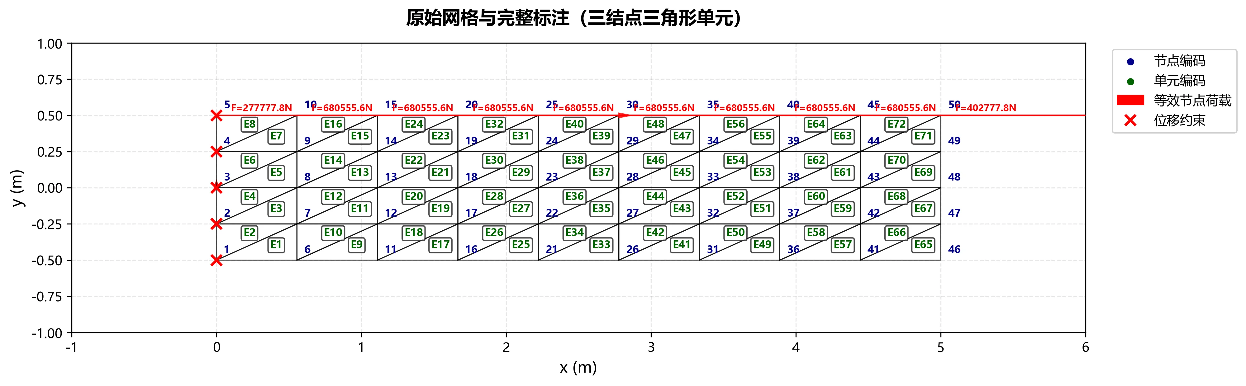
"""
保存图1:原始网格与完整标注(单元/节点/荷载/约束)"""
fig, ax = plt.subplots(figsize=(14, 8))
ax.set_title('原始网格与完整标注(单元/节点/荷载/约束)', fontsize=14, fontweight='bold', pad=15)
ax.set_xlabel('x (m)', fontsize=12)
ax.set_ylabel('y (m)', fontsize=12)
for i in range(nx):
ax.plot(node_x[i, :], node_y[i, :], 'k-', linewidth=0.8, alpha=0.7)
for j in range(ny):
ax.plot(node_x[:, j], node_y[:, j], 'k-', linewidth=0.8, alpha=0.7)
node_flat_x = node_x.flatten()
node_flat_y = node_y.flatten()
for node_idx in range(nx*ny):
ax.text(
node_flat_x[node_idx] + 0.05, node_flat_y[node_idx] + 0.05,
f"{node_idx+1}", fontsize=8, color='darkblue', fontweight='bold'
)
for elem_id, elem_nodes in enumerate(elem_conn):
elem_node_idx = [n-1 for n in elem_nodes]
elem_center_x = np.mean(node_flat_x[elem_node_idx])
elem_center_y = np.mean(node_flat_y[elem_node_idx])
ax.text(
elem_center_x, elem_center_y, f"E{elem_id+1}",
fontsize=9, color='darkgreen', fontweight='bold',
bbox=dict(boxstyle="round,pad=0.2", facecolor='white', alpha=0.7)
)
arrow_length_scale = 1e-5
for i, node_idx in enumerate(top_nodes):
load_x = global_load[2*node_idx, 0]
if abs(load_x) > TINY_VALUE:
ax.arrow(
node_flat_x[node_idx], node_flat_y[node_idx],
load_x * arrow_length_scale, 0,
head_width=0.03, head_length=0.08, fc='red', ec='red', alpha=0.8, zorder=5
)
ax.text(
node_flat_x[node_idx] + 0.1, node_flat_y[node_idx] + 0.03,
f"F={load_x:.1f}N", fontsize=7, color='red', fontweight='bold'
)
for node_idx in fixed_nodes:
ax.plot(
node_flat_x[node_idx], node_flat_y[node_idx],
'rx', markersize=8, markeredgewidth=2, zorder=6
)
ax.scatter([], [], c='darkblue', label='节点编码', s=20)
ax.scatter([], [], c='darkgreen', label='单元编码', s=20)
ax.arrow(0, 0, 0, 0, fc='red', ec='red', label='等效节点荷载', head_width=0.03)
ax.plot([], [], 'rx', markersize=8, markeredgewidth=2, label='位移约束')
ax.legend(loc='upper left', bbox_to_anchor=(1.02, 1), fontsize=10, framealpha=0.9)
ax.set_aspect('equal')
ax.grid(True, alpha=0.3, linestyle='--')
ax.set_xlim(-1.0, BEAM_LENGTH + 1.0)
ax.set_ylim(-1.0, 1.0)
filename = f'悬臂梁_原始网格_完整标注_{nx}x{ny}.png'
plt.savefig(filename, dpi=300, bbox_inches='tight')
print(f"已保存: {filename}")
plt.close()
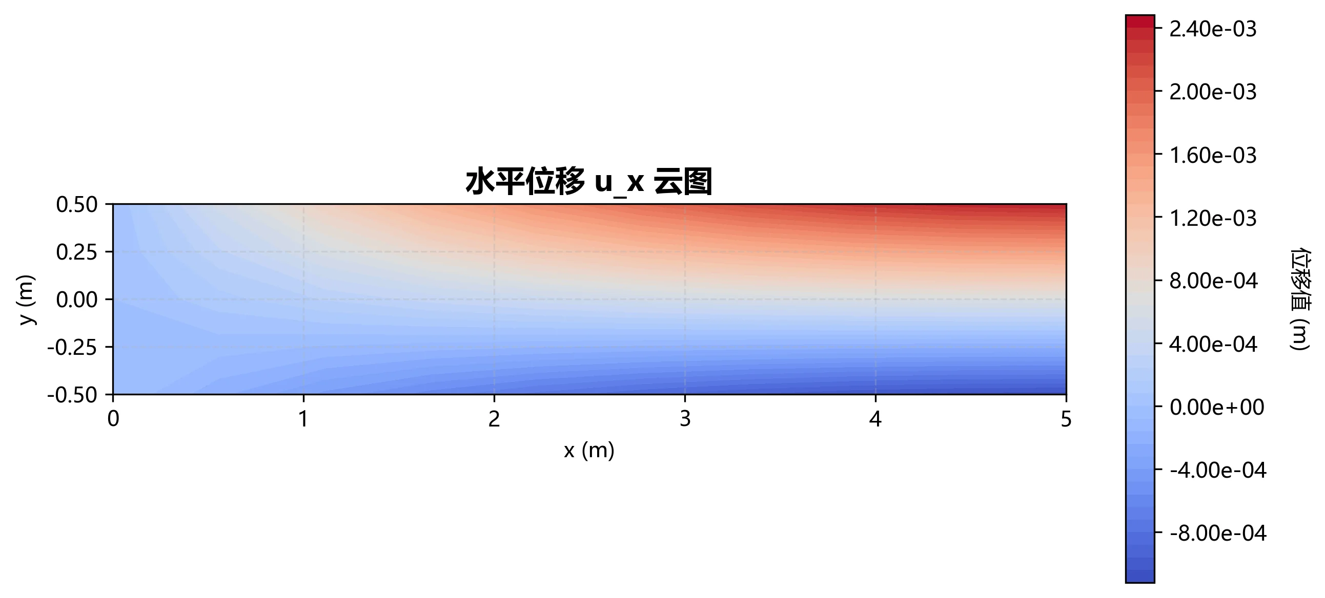
def save_disp_x_plot(node_x: np.ndarray, node_y: np.ndarray, disp_x: np.ndarray, nx: int, ny: int) -> None:
"""保存图2:水平位移云图"""
fig, ax = plt.subplots(figsize=(10, 6))
disp_contour = disp_x.reshape(nx, ny)
contour = ax.contourf(node_x, node_y, disp_contour, levels=50, cmap='coolwarm')
ax.set_title('水平位移 u_x 云图', fontsize=14, fontweight='bold')
ax.set_xlabel('x (m)')
ax.set_ylabel('y (m)')
cbar = plt.colorbar(contour, ax=ax, format='%.2e', shrink=0.8)
cbar.set_label('位移值 (m)', rotation=270, labelpad=20)
ax.set_aspect('equal')
ax.grid(True, alpha=0.3, linestyle='--')
filename = f'悬臂梁_水平位移_{nx}x{ny}.png'
plt.savefig(filename, bbox_inches='tight')
print(f"已保存: {filename}")
plt.close()
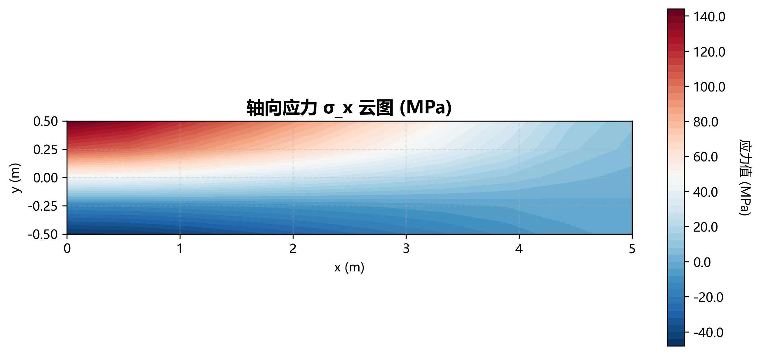
def save_stress_x_plot(node_x: np.ndarray, node_y: np.ndarray, stress_x: np.ndarray, nx: int, ny: int) -> None:
"""保存图3:轴向应力云图"""
fig, ax = plt.subplots(figsize=(10, 6))
stress_contour = stress_x.reshape(nx, ny)
contour = ax.contourf(node_x, node_y, stress_contour, levels=50, cmap='RdBu_r')
ax.set_title('轴向应力 σ_x 云图 (MPa)', fontsize=14, fontweight='bold')
ax.set_xlabel('x (m)')
ax.set_ylabel('y (m)')
cbar = plt.colorbar(contour, ax=ax, format='%.1f', shrink=0.8)
cbar.set_label('应力值 (MPa)', rotation=270, labelpad=20)
ax.set_aspect('equal')
ax.grid(True, alpha=0.3, linestyle='--')
filename = f'悬臂梁_轴向应力_{nx}x{ny}.png'
plt.savefig(filename, bbox_inches='tight')
print(f"已保存: {filename}")
plt.close()
def save_deformed_mesh_plot(
node_x: np.ndarray,
node_y: np.ndarray,
def_x: np.ndarray,
def_y: np.ndarray,
nx: int,
ny: int
) -> None:
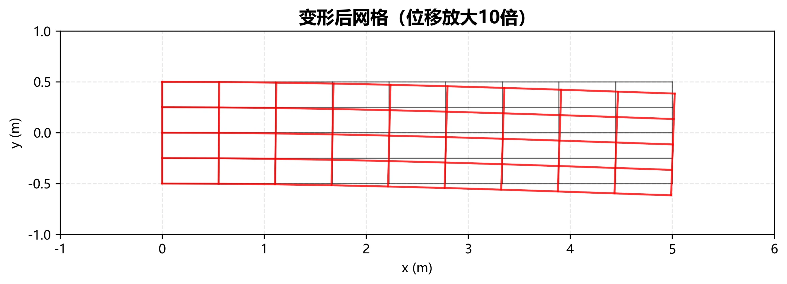
"""保存图4:变形后网格 """
fig, ax = plt.subplots(figsize=(10, 6))
ax.set_title(f'变形后网格(位移放大{DISP_SCALE_FACTOR}倍)', fontsize=14, fontweight='bold')
ax.set_xlabel('x (m)')
ax.set_ylabel('y (m)')
for i in range(nx):
ax.plot(node_x[i, :], node_y[i, :], 'k-', linewidth=0.8, alpha=0.6)
for j in range(ny):
ax.plot(node_x[:, j], node_y[:, j], 'k-', linewidth=0.8, alpha=0.6)
def_x_scaled = node_x + (def_x - node_x) * DISP_SCALE_FACTOR
def_y_scaled = node_y + (def_y - node_y) * DISP_SCALE_FACTOR
for i in range(nx):
ax.plot(def_x_scaled[i, :], def_y_scaled[i, :], 'r-', linewidth=1.5, alpha=0.8)
for j in range(ny):
ax.plot(def_x_scaled[:, j], def_y_scaled[:, j], 'r-', linewidth=1.5, alpha=0.8)
ax.set_aspect('equal')
ax.grid(True, alpha=0.3, linestyle='--')
ax.set_xlim(-1.0, BEAM_LENGTH + 1.0)
ax.set_ylim(-1.0, 1.0)
filename = f'悬臂梁_变形网格_{nx}x{ny}.png'
plt.savefig(filename, bbox_inches='tight')
print(f"已保存: {filename}")
plt.close()
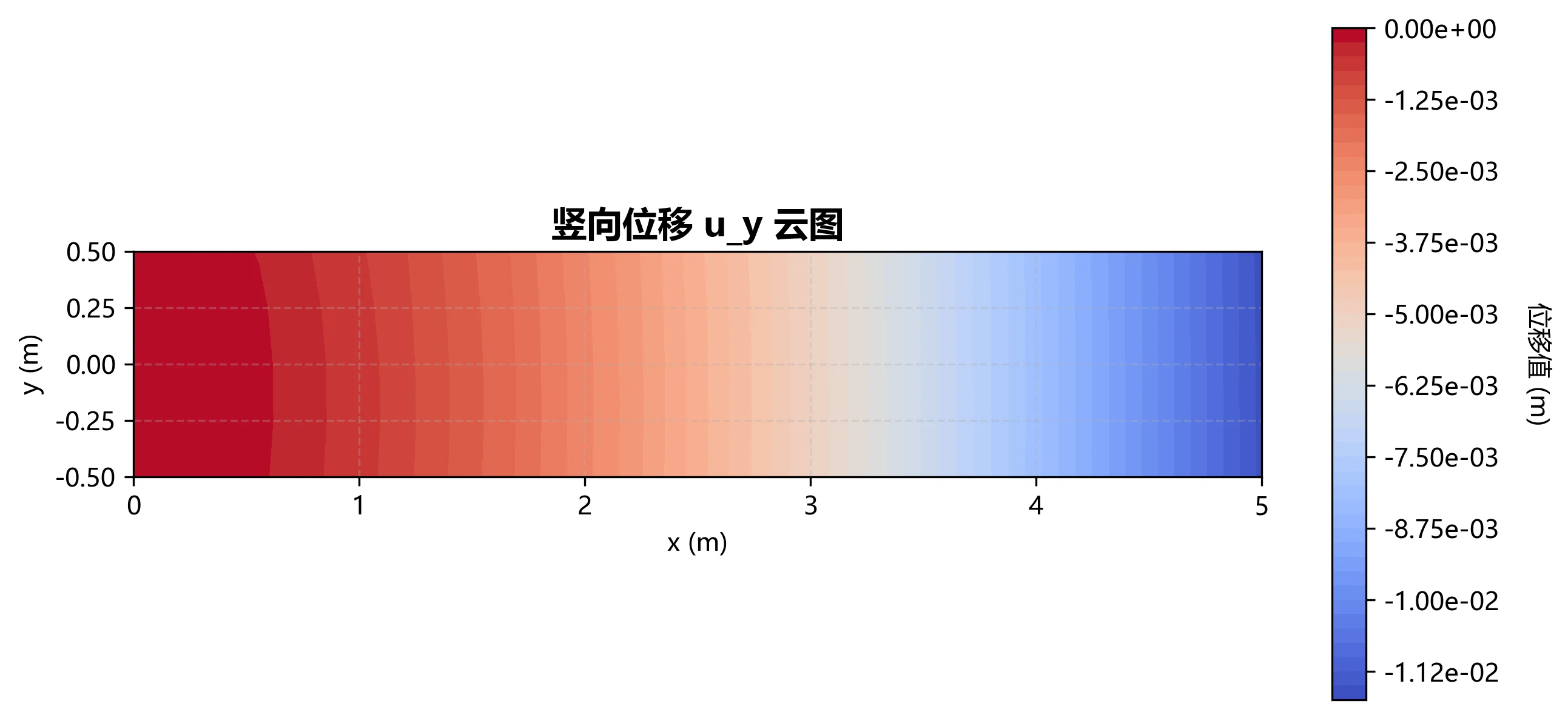
def save_disp_y_plot(node_x: np.ndarray, node_y: np.ndarray, disp_y: np.ndarray, nx: int, ny: int) -> None:
"""保存图5:竖向位移云图"""
fig, ax = plt.subplots(figsize=(10, 6))
disp_contour = disp_y.reshape(nx, ny)
contour = ax.contourf(node_x, node_y, disp_contour, levels=50, cmap='coolwarm')
ax.set_title('竖向位移 u_y 云图', fontsize=14, fontweight='bold')
ax.set_xlabel('x (m)')
ax.set_ylabel('y (m)')
cbar = plt.colorbar(contour, ax=ax, format='%.2e', shrink=0.8)
cbar.set_label('位移值 (m)', rotation=270, labelpad=20)
ax.set_aspect('equal')
ax.grid(True, alpha=0.3, linestyle='--')
filename = f'悬臂梁_竖向位移_{nx}x{ny}.png'
plt.savefig(filename, bbox_inches='tight')
print(f"已保存: {filename}")
plt.close()
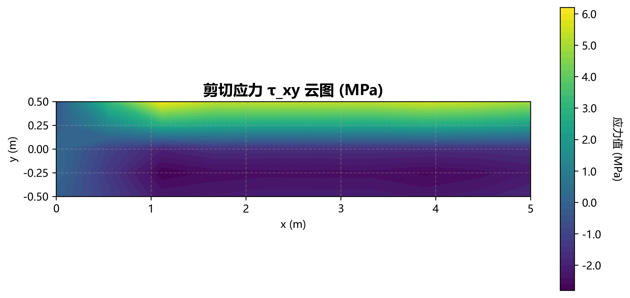
def save_stress_xy_plot(node_x: np.ndarray, node_y: np.ndarray, stress_xy: np.ndarray, nx: int, ny: int) -> None:
"""保存图6:剪切应力云图"""
fig, ax = plt.subplots(figsize=(10, 6))
stress_contour = stress_xy.reshape(nx, ny)
contour = ax.contourf(node_x, node_y, stress_contour, levels=50, cmap='viridis')
ax.set_title('剪切应力 τ_xy 云图 (MPa)', fontsize=14, fontweight='bold')
ax.set_xlabel('x (m)')
ax.set_ylabel('y (m)')
cbar = plt.colorbar(contour, ax=ax, format='%.1f', shrink=0.8)
cbar.set_label('应力值 (MPa)', rotation=270, labelpad=20)
ax.set_aspect('equal')
ax.grid(True, alpha=0.3, linestyle='--')
filename = f'悬臂梁_剪切应力_{nx}x{ny}.png'
plt.savefig(filename, bbox_inches='tight')
print(f"已保存: {filename}")
plt.close()
def run_fea_analysis() -> Dict[str, Any]:
"""悬臂梁平面应力有限元分析主函数"""
print("="*60)
print("等截面悬臂梁平面应力有限元分析程序 v2.4")
print("="*60)
try:
print("\n[1/6] 输入网格参数")
print("-"*40)
nx = get_valid_integer_input("水平方向节点数(≥2): ")
ny = get_valid_integer_input("竖直方向节点数(≥2): ")
ne_x = nx - 1
ne_y = ny - 1
n_nodes = nx * ny
n_elems = ne_x * ne_y
print(f"\n网格信息:")
print(f" 节点数: {n_nodes} ({nx}×{ny}) | 单元数: {n_elems} ({ne_x}×{ne_y})")
print(f" 提示:增加节点数可降低计算误差")
print("\n[2/6] 材料与几何参数")
print("-"*40)
print(f"几何参数:长度={BEAM_LENGTH}m | 高度={BEAM_HEIGHT}m | 厚度={BEAM_THICKNESS}m")
print(f"材料参数:E={ELASTIC_MODULUS:.4e}Pa | ν={POISSON_RATIO} | 剪应力={APPLIED_SHEAR_STRESS:.4e}Pa")
print("\n[3/6] 理论解")
print("-"*40)
theory = {
"自由端水平位移(m)": THEORY_DISP_X,
"自由端竖向位移(m)": THEORY_DISP_Y
}
for k, v in theory.items():
print(f" {k}: {v:.8e}")
print("\n[4/6] 生成有限元网格")
print("-"*40)
node_x = np.zeros((nx, ny), dtype=FLOAT_TYPE)
node_y = np.zeros((nx, ny), dtype=FLOAT_TYPE)
x_coords = np.linspace(0, BEAM_LENGTH, nx, dtype=FLOAT_TYPE)
y_coords = np.linspace(-BEAM_HEIGHT/2, BEAM_HEIGHT/2, ny, dtype=FLOAT_TYPE)
for i in range(nx):
node_x[i, :] = x_coords[i]
for j in range(ny):
node_y[:, j] = y_coords[j]
print(f"坐标范围:x=[{node_x.min():.6f}, {node_x.max():.6f}]m | y=[{node_y.min():.6f}, {node_y.max():.6f}]m")
elem_conn = []
for i in range(ne_x):
for j in range(ne_y):
n1 = i * ny + j + 1
n2 = (i+1) * ny + j + 1
n3 = (i+1) * ny + j + 2
n4 = i * ny + j + 2
elem_conn.append([n1, n2, n3, n4])
D = (ELASTIC_MODULUS / (1 - POISSON_RATIO**2)) * np.array([
[1, POISSON_RATIO, 0],
[POISSON_RATIO, 1, 0],
[0, 0, (1-POISSON_RATIO)/2]
], dtype=FLOAT_TYPE)
gauss_pts, gauss_wts = leggauss(GAUSS_ORDER)
print("\n[5/6] 组装刚度矩阵与荷载向量")
print("-"*40)
K = np.zeros((2*n_nodes, 2*n_nodes), dtype=FLOAT_TYPE)
F = np.zeros((2*n_nodes, 1), dtype=FLOAT_TYPE)
for elem_id, elem_nodes in enumerate(elem_conn):
if (elem_id+1) % max(1, n_elems//10) == 0:
progress = (elem_id+1)/n_elems*100
print(f" 处理单元 {elem_id+1}/{n_elems} ({progress:.0f}%)")
elem_idx = [n-1 for n in elem_nodes]
elem_x = node_x.flatten()[elem_idx]
elem_y = node_y.flatten()[elem_idx]
is_top_elem = np.max(elem_y) >= (BEAM_HEIGHT/2 - TINY_VALUE)
ke = np.zeros((8, 8), dtype=FLOAT_TYPE)
for i in range(GAUSS_ORDER):
for j in range(GAUSS_ORDER):
s = gauss_pts[i]
t = gauss_pts[j]
dN_ds, dN_dt = quad4_shape_derivatives(s, t)
jac, det_jac, inv_jac = calculate_jacobian(dN_ds, dN_dt, elem_x, elem_y)
dN_dx = inv_jac[0,0]*dN_ds + inv_jac[0,1]*dN_dt
dN_dy = inv_jac[1,0]*dN_ds + inv_jac[1,1]*dN_dt
B = calculate_B_matrix(dN_dx, dN_dy)
weight = gauss_wts[i] * gauss_wts[j] * det_jac * BEAM_THICKNESS
ke += B.T @ D @ B * weight
if is_top_elem:
fe = calculate_surface_load(elem_x, elem_y, APPLIED_SHEAR_STRESS, BEAM_THICKNESS)
for local_i, global_i in enumerate(elem_idx):
F[2*global_i, 0] += fe[2*local_i]
F[2*global_i+1, 0] += fe[2*local_i+1]
for local_i, global_i in enumerate(elem_idx):
for local_j, global_j in enumerate(elem_idx):
K[2*global_i:2*global_i+2, 2*global_j:2*global_j+2] += ke[2*local_i:2*local_i+2, 2*local_j:2*local_j+2]
total_load = np.sum(F)
theory_load = APPLIED_SHEAR_STRESS * BEAM_THICKNESS * BEAM_LENGTH
print(f"\n荷载信息:")
print(f" 总施加荷载: {total_load:.6f}N | 理论总荷载: {theory_load:.6f}N")
print(f" 荷载误差: {abs(total_load - theory_load):.6e}N")
print("\n[6/6] 求解位移与应力")
print("-"*40)
fixed_nodes = list(range(ny))
fixed_dofs = []
for n in fixed_nodes:
fixed_dofs.append(2*n)
fixed_dofs.append(2*n+1)
free_dofs = [d for d in range(2*n_nodes) if d not in fixed_dofs]
K_red = K[np.ix_(free_dofs, free_dofs)]
F_red = F[free_dofs, :]
cond_num = np.linalg.cond(K_red)
print(f"刚度矩阵条件数: {cond_num:.2e}")
if cond_num > 1e10:
print("警告:条件数较大,建议加密网格")
u_red = np.linalg.solve(K_red, F_red)
u = np.zeros((2*n_nodes, 1), dtype=FLOAT_TYPE)
u[free_dofs, :] = u_red
disp_x = u[::2].flatten()
disp_y = u[1::2].flatten()
print(f"\n位移范围:")
print(f" 水平位移: [{disp_x.min():.8e}, {disp_x.max():.8e}]m")
print(f" 竖向位移: [{disp_y.min():.8e}, {disp_y.max():.8e}]m")
print("\n后处理:提取自由端中点位移")
print("-"*40)
fem_dx, fem_dy = get_free_end_mid_disp(u, node_x, node_y)
fem = {
"自由端水平位移(m)": fem_dx,
"自由端竖向位移(m)": fem_dy
}
print(f" 水平位移: {fem_dx:.8e}m | 竖向位移: {fem_dy:.8e}m")
print("\n后处理:计算单元应力")
print("-"*40)
elem_stress = np.zeros((n_elems, 3), dtype=FLOAT_TYPE)
for elem_id, elem_nodes in enumerate(elem_conn):
elem_idx = [n-1 for n in elem_nodes]
ue = np.zeros(8, dtype=FLOAT_TYPE)
for local_i, global_i in enumerate(elem_idx):
ue[2*local_i] = u[2*global_i, 0]
ue[2*local_i+1] = u[2*global_i+1, 0]
elem_x = node_x.flatten()[elem_idx]
elem_y = node_y.flatten()[elem_idx]
stress_avg = np.zeros(3, dtype=FLOAT_TYPE)
count = 0
for i in range(GAUSS_ORDER):
for j in range(GAUSS_ORDER):
count += 1
s = gauss_pts[i]
t = gauss_pts[j]
dN_ds, dN_dt = quad4_shape_derivatives(s, t)
jac, det_jac, inv_jac = calculate_jacobian(dN_ds, dN_dt, elem_x, elem_y)
dN_dx = inv_jac[0,0]*dN_ds + inv_jac[0,1]*dN_dt
dN_dy = inv_jac[1,0]*dN_ds + inv_jac[1,1]*dN_dt
B = calculate_B_matrix(dN_dx, dN_dy)
strain = B @ ue
stress = D @ strain
stress_avg += stress
elem_stress[elem_id, :] = stress_avg / count
print(f"应力范围:")
print(f" 轴向应力: [{elem_stress[:,0].min():.4e}, {elem_stress[:,0].max():.4e}]Pa")
print(f" 剪切应力: [{elem_stress[:,2].min():.4e}, {elem_stress[:,2].max():.4e}]Pa")
print_result_compare(theory, fem)
dx_err = abs((fem_dx - THEORY_DISP_X)/THEORY_DISP_X)*100
dy_err = abs((fem_dy - THEORY_DISP_Y)/THEORY_DISP_Y)*100
print(f"\n误差分析:")
print(f" 水平位移相对误差: {dx_err:.4f}%")
print(f" 竖向位移相对误差: {dy_err:.4f}%")
if dx_err < 1.0:
print(f" ✅ 水平位移误差<1%,满足工程精度要求")
print("\n生成可视化结果")
print("-"*40)
def_x = node_x.flatten() + disp_x
def_y = node_y.flatten() + disp_y
def_x = def_x.reshape(nx, ny)
def_y = def_y.reshape(nx, ny)
node_stress_x = np.zeros(n_nodes, dtype=FLOAT_TYPE)
node_stress_xy = np.zeros(n_nodes, dtype=FLOAT_TYPE)
node_count_x = np.zeros(n_nodes, dtype=int)
node_count_xy = np.zeros(n_nodes, dtype=int)
for elem_id, elem_nodes in enumerate(elem_conn):
sx = elem_stress[elem_id, 0]
sxy = elem_stress[elem_id, 2]
for n in elem_nodes:
idx = n-1
node_stress_x[idx] += sx
node_stress_xy[idx] += sxy
node_count_x[idx] += 1
node_count_xy[idx] += 1
node_stress_x_avg = node_stress_x / node_count_x / 1e6
node_stress_xy_avg = node_stress_xy / node_count_xy / 1e6
top_nodes = [i*ny + (ny-1) for i in range(nx)]
print("\n保存图片文件:")
print("-"*40)
save_mesh_plot_with_annotations(node_x, node_y, top_nodes, elem_conn, F, fixed_nodes, nx, ny)
save_disp_x_plot(node_x, node_y, disp_x, nx, ny)
save_stress_x_plot(node_x, node_y, node_stress_x_avg, nx, ny)
save_deformed_mesh_plot(node_x, node_y, def_x, def_y, nx, ny)
save_disp_y_plot(node_x, node_y, disp_y, nx, ny)
save_stress_xy_plot(node_x, node_y, node_stress_xy_avg, nx, ny)
return {
'nodal_displacements': u,
'element_stresses': elem_stress,
'mesh_info': {'nx': nx, 'ny': ny, 'n_nodes': n_nodes, 'n_elems': n_elems},
'theory_solution': theory,
'fem_solution': fem,
'error': {'dx_err': dx_err, 'dy_err': dy_err}
}
except Exception as e:
print(f"\n程序执行错误: {str(e)}")
traceback.print_exc()
return None
if __name__ == "__main__":
results = run_fea_analysis()
if results:
print("\n✅ 悬臂梁有限元分析完成!")
if results['error']['dx_err'] < 1.0:
print(f"📊 水平位移相对误差 {results['error']['dx_err']:.4f}%,达到高精度要求")
else:
print("\n❌ 程序执行失败,请检查错误信息")
|


 - Primerusse's Utopia&pics=/assets/pictures/article_illustrations/decorations/LiuLiShenShe_202512_11.webp&summary=第1章 悬臂梁平面问题题目
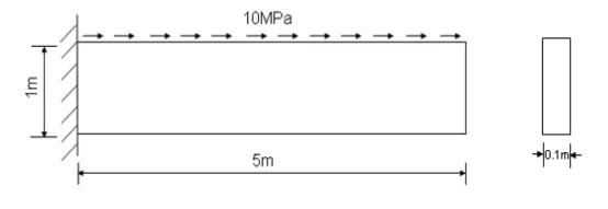
图1.1 悬臂梁示意图
已知:悬臂梁的材料参数为E=190GPaE=190GPaE=190GPa,μ=0.25\mu=0.25μ=0.25,t=10cmt=10cmt=10cm,ρ=0\rho=0ρ=...)

